An autoregression model from scratch for forecasting the number of academic publications pre- and post- COVID-19 pandemic
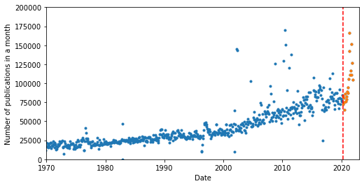
Previously I showed that 2021 was a bumper year for academic publications, suggesting that the changes in working practices brought about by COVID-19 had caused an increase in publication rates.
The time series that I created for this work seemed like a great test bed to familiarise myself with autoregression, a common forecasting method, and to further validate the conclusions on the impact of COVID-19 to research output.
An autoregressive model assumes that there is a common relationship between previous and subsequent data points. For example, consider annnual interest paid on an account, the forecast amount for next year is just this years amount plus the amount times the interest rate. Here, the interest rate is the common factor to forecast the amount we will have next year and can be used to iteratively calculate the amount in the account for future years. This is for a lag of 1, since we only use the previous date point to do the forecast, but there could be relationships with lags of 2, 3, 4 etc. for the forecast. By combining all these terms we can capture the time-series with seasonality of different timescales.
The mathematical description of this process is:
X(t+1) = p_0 + p_1*X(t-1) + p_2*X(t-2) + ... + p_n*X(t-n)
Where p_0 to p_n are autoregression components which are obtained by fitting and there is one for every lag period included in the model.
Since this is a learning excersise, I want to implement the algorithm from scratch. However, there are plenty of modules out there that can do this in a line or two of code, including statsmodels.
We still need a few imports though:
import pandas as pd
import numpy as np
from scipy.optimize import curve_fit
import matplotlib.pyplot as plt
import datetime as dt
I saved the monthly publications data as a csv. You can download it from here.
df_pubs = pd.read_csv('pubs_by_year.csv', index_col=0)
df_pubs.columns = ['date', 'n_publications']
df_pubs.date = pd.to_datetime(df_pubs.date, format='%Y/%m/%d').dt.date
df_pubs.set_index('date', inplace=True)
I will filter the data as before, removing extreme outliers that are more than 3 standard deviations from the mean monthly number of publications. I will also create a new dataframe which contains the post lockdown publications.
df_pubs['z_score'] = (df_pubs.n_publications - df_pubs.n_publications.mean())/df_pubs.n_publications.std()

mn = df_pubs.n_publications.mean()
df_pubs.loc[df_pubs.z_score.abs() > 3, 'n_publications'] = mn # Filter out datapoints with a z-score more than 4
df_pubs_post_covid = df_pubs.iloc[663:].copy()  # Post UK lockdown indexes on filtered data
Plotting up the data as before:
uk_lockdown_date = dt.date(2020,3,27)

fig = plt.figure(figsize=(8,4))
plt.plot(df_pubs.index, df_pubs['n_publications'], '.')
plt.plot(df_pubs_post_covid.index, df_pubs_post_covid['n_publications'], '.')
plt.ylim([0,200000])
plt.xlim([dt.date(1970,1,1), dt.date(2023,1,1)])
plt.ylabel('Number of publications in a month')
plt.xlabel('Date')
plt.plot([uk_lockdown_date, uk_lockdown_date],[0, 500e3], '--r', label='First UK lockdown announced')

For an autoregressive model to work, there needs to be a correlation between prior datapoints and future datapoints. We want to see if there is a relationship between common lags between datapoints i.e. lags of 12 months, 24 months etc. and therefore if we can use these to predict the number of publications in the future.
We do this with lag plots and there is a handy tool in pandas for generating these plots:
fig, ax = plt.subplots(nrows=1, ncols=4, figsize=(16,4), sharex=True, sharey=True)
# plt.xlim([-40e3, 80e3])
# plt.ylim([-40e3, 80e3])
pd.plotting.lag_plot(df_pubs.n_publications, lag=6, ax=ax[0])
pd.plotting.lag_plot(df_pubs.n_publications, lag=12, ax=ax[1])
pd.plotting.lag_plot(df_pubs.n_publications, lag=18, ax=ax[2])
pd.plotting.lag_plot(df_pubs.n_publications, lag=24, ax=ax[3])

There is a good positive correlation in the above figures, so we can proceed with an autoregressive model.
In the following, I create the auto_regression class with the tools to model our time series. There are various components to this:
-
estimate_trend_and_subtract: Before modeling any time series we need to make sure it is stationary, which means that the mean shouldn’t be changing with time i.e. no trend or seasonality. There are a number of ways to do this, and various tests that exist to confirm the dataset is stations (e.g. Dicky-Fuller test), but in this example I’ll take the simplest approach which is to subtract a rolling mean. -
train_test_split: This method splits the data into training and test data. In this case we will split in the date the UK went into lockdown to see if the trend post lockdown can be capture by what our model has learnt from the pre-pandemic publication rate. -
generate_lags: This method creates the lagged data that will be the input for out model. There will be a new column for each lag period, which will be the monthly publications data, but shifted out of time by lag length. -
fit_AR_model: This does a least squares minimisation to find the autoregression components. These autoregression component are related to the gradient of the above lag plots i.e. what constant connects the y(-12months) data to y(today) - but for every lagged dataset in our model, not just the four the I showed above. The scipy curve_fit model need to be fed a function, hence why the linear_function method is there, which is just the product of the lagged data and the fitting parameter. -
forecast_future: This method uses the autoregression components obtained above to predict a future month’s number of publications. This will be stationary though, so it uses this new value with the historical data to calculate the trend, which is added back in to obtain the forecast number of publications for that month. With this new value we can calculate the corresponded lagged data and append the completed row onto our dataset. In this way we can iteratively step through the future months creating a forecast for any data in the future.
class auto_regression:
    def __init__(self, df):
        self.df_pubs = pd.DataFrame(df)

    def estimate_trend_and_subtract(self, window=24):
        self.df_pubs['trend'] = self.df_pubs.n_publications.rolling(window=window).mean().fillna(0)
        self.df_pubs['stationary'] = self.df_pubs.n_publications-self.df_pubs.trend # df_pubs.n_publications.shift(1)

    def train_test_split(self, split_date):
        # Split our data into train and test datasets. Dividing before and after first UK lockdown.
        cols = self.df_pubs.columns
        X_train = self.df_pubs[self.df_pubs.index < split_date][cols[3:]]   # nb/ don't use the first 3 cols as these don't contain the lags
        y_train = self.df_pubs[self.df_pubs.index < split_date]['stationary']
        X_test = self.df_pubs[self.df_pubs.index > split_date][cols[3:]]
        y_test = self.df_pubs[self.df_pubs.index > split_date]['stationary']
        return X_train, y_train, X_test, y_test

    def generate_lags(self, df_pubs, start, end, step):
        lags = np.arange(start, end, step)
        for i in lags:
            self.df_pubs['lag_{0}'.format(i)] = self.df_pubs['stationary'].shift(i)

        self.df_pubs.fillna(0, inplace=True)

    def fit_AR_model(self, X_train, y_train, p0):
        popt, _ = curve_fit(self.linear_function, X_train, y_train, p0=p0)
        return popt

    def linear_function(self, x, *args):
        a = args
        return x@a

    def forecast_future(self, df_pubs, future, popt, window):
        cols = self.df_pubs.columns
        lag_cols = cols[cols.str.contains('lag')]
        for month in future:
            df_next_month = pd.DataFrame(columns=cols, data=[np.zeros(len(cols))])
            df_next_month['stationary'] = self.df_pubs[lag_cols].iloc[-1]@popt  # Forecast next month based on our model applied to the previous data point.

            #  Calculate the trend on this date using the 'moving' average of the historic and forecast data within this window
            df_next_month['trend'] = self.df_pubs.iloc[-window:].n_publications.mean()

            # Add the trend to the stationary component to get the forecast publications
            df_next_month['n_publications'] = df_next_month['stationary'] + df_next_month['trend']

            # Even though this df has just one row, we need to give it an index so the concat later works.
            df_next_month.index = [month.date()]
            # Calculate the lags for this month using the forecast publications.
            lags = np.arange(start, end, step)
            for i in lags:
                df_next_month['lag_{0}'.format(i)] = self.df_pubs.shift(i).stationary.iloc[-1] # Calculate the new lags for this future month
            # Append this forecast month onto the df_pubs dataframe so that when the process repeats the forecast data will be included in the moving average, lags etc.
            self.df_pubs = pd.concat([self.df_pubs, df_next_month])
The class is applied to fit an autoregression model in the following code block:
ar = auto_regression(df=df_pubs['n_publications']) # Create an auto_regression object

window = 24
ar.estimate_trend_and_subtract(window=window) # Subtract the trend to make the data stationary

start = 12 # months
step = 12
end = step*10  # Look back 10 years

ar.generate_lags(df_pubs, start, end, step) # Generate the lagged data to be used when fitting the model
X_train, y_train, X_test, y_test = ar.train_test_split(split_date=uk_lockdown_date)

p0 = np.ones(9)  # Initialise our autoregressive coefficients
popt = ar.fit_AR_model(X_train, y_train, p0)   # Fit the AR model to our training data
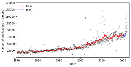
Now I visualise the fit and it’s not too bad:
fig = plt.figure(figsize=(8,4))
y_train_trend = ar.df_pubs[ar.df_pubs.index < uk_lockdown_date]['trend'] # Split the trend data into training and test to aid the visualisation
y_test_trend = ar.df_pubs[ar.df_pubs.index > uk_lockdown_date]['trend']

# Note the model returns the predicted stationary data, so the trend has to be added back in to compare to the experimental data
plt.plot(X_train.index, y_train + y_train_trend, 'k.', alpha=0.3)
plt.plot(X_train@popt + y_train_trend, 'r-', label='train')

plt.plot(X_test.index, y_test + y_test_trend, 'k.', alpha=0.3)
plt.plot(X_test@popt + y_test_trend, 'b-', label='test')

plt.legend()
plt.ylim([0,200000])
plt.xlim([dt.date(1970,1,1), dt.date(2023,1,1)])
plt.ylabel('Number of publications in a month')
plt.xlabel('Date')

Now let’s use this model to forecast into the future:
future = pd.date_range(start='2022-01-01', periods=12*5, freq='MS') # Create a dataframe of the dates in the future we want to forecast for
We iteratively forecast one month in the future, then use this new data to produce the new lags to forecast the month after (and so forth…)
future = pd.date_range(start='2022-01-01', periods=12*5, freq='MS')  # Future is just a list of dates in the future which we want to forecast.
ar.forecast_future(df_pubs, future, popt, window)  # Do the forecast
df_future = ar.df_pubs.tail(len(future))  # Extract the forecast part of the dataframe
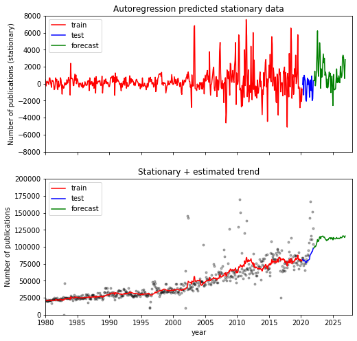
Now plot the results. At the top I’ve plotted the stationary data as output from the model, and below with the combined stationary + trend data to compare with the actual data. It’s interesting the observe the sudden change in slope in the test data which encompasses the pandemic followed by a return to the more gentle rise in publications for the forecast.
fig, ax = plt.subplots(nrows=2, ncols=1, figsize=(8, 8), sharex=True)

# Raw stationary values:
fig = plt.figure(figsize=(8,4))
ax[0].plot(X_train@popt , 'r-', label='train')

ax[0].plot(X_test@popt, 'b-', label='test')

ax[0].plot(df_future.index, df_future.stationary, 'g-', label='forecast')
ax[0].set_xlim([dt.date(1980,1,1), dt.date(2028,1,1)])
ax[0].set_ylim([-8e3,8e3])
ax[0].set_title('Autoregression predicted stationary data')
ax[0].set_ylabel('Number of publications (stationary)')
ax[0].legend()

# With the trend added back in:
ax[1].plot(X_train.index, y_train + y_train_trend, 'k.', alpha=0.3)
ax[1].plot(X_train@popt + y_train_trend, 'r-', label='train')

ax[1].plot(X_test.index, y_test + y_test_trend, 'k.', alpha=0.3)
ax[1].plot(X_test@popt + y_test_trend, 'b-', label='test')

ax[1].plot(df_future.index, df_future.stationary + df_future.trend, 'g-', label='forecast')
ax[1].set_ylim([0,200000])
ax[1].set_xlim([dt.date(1980,1,1), dt.date(2028,1,1)])
ax[1].set_title('Stationary + estimated trend')
ax[1].set_xlabel('year')
ax[1].set_ylabel('Number of publications')
ax[1].legend()

This is really a very simple model and ultimately just a bit of fun, but I’m surprised as to how it has captured differing behaviour for pre and post pandemic and it will be interesting to see whether the publication rate in the future does indeed follow this behaviour.
